Determining an Equilibrium Constant
Jarrod Cook
15 October 2004
Block 3
Partner: Kareem Syed
Objectives:
The objective of this lab is to find the equilibrium constant of Fe(SCN)2+ through multiple trials using a spectrometer. This able will develop skills and teach practical uses for the spectrometer. LeChatelier’s principle will demonstrated in this lab and a better understanding will be formed. Since one chemical is colorless and the other is colored a spectrometer can be used to monitor amounts of each in the solution. By completing multiple trials an average can be reached for the value of the equilibrium constant of Fe(SCN)2+.
Procedures:
To complete this lab several chemicals must be measured and transferred to test tubes. First 4.0 ml of 0.0025 M Fe(NO3)3 must be diluted to a total volume of 100 ml in a volumetric flask. This solution is then added to 5 test tubes in 1 mm increments. Next 5 mm of 1 M KSCN is added to the solution and then each test tube is given equal amounts of volume by adding 0.1 M HNO3. Each test tube is then put in to cuvets and tested in the spectrometer at 450 nm and the absorbance is recorded.
In the second part of this lab the same process will be used but with different amounts of substances. This time the 0.0025 Fe(NO3)3 and KSCN will be used, the HNO3 will remain the same. Five test tubes will be filled with 1.0 ml of Fe(NO3)3 and five more will be filled with 2.0 ml of the substance. Each set of five test tubes will be filled with 0.5 ml increments of KSCN starting at 1.0 ml and ending at 3.0 ml. The test tubes will then once again be given equal volumes by adding the required amount of HNO3. The solutions will once again be transferred to cuvets and put in a spectrometer at 450 nm. Once their absorbance has been recorded the procedures are complete.
Conclusions:
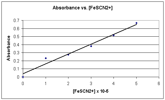
This lab was very extensive and clearly demonstrated the process of determining equilibrium constant. After working through many calculations I came out with an average constant of 154.3, an accurate measurement. Although my readings caused me to have an accurate final answer, they were not precise. My values for the equilibrium constant varied greatly in some of ten trials, ranging from a low of 28.9 to a high of 421. The cause for these incorrect readings was most likely human error, such as incorrect measurement. Other contributions to the value of the constant would be the accuracy of the measuring devices, the purity of the solution and the accuracy of the best-fit line drawn on the graph. Since one of these solutions is clear and the other is colored their Concentrations can easily be found. The solutions can be simply put into a spectrometer and the absorbance will reveal how much of the colored solution resides in the solution. Your results in part one of the experiment can be used to create a graph with which you can make a best fit line and find values for the absorbencies in part two. This information can then be used to calculate the equilibrium constant in all or ten trials and an average can be taken. LeChatelier’s principle takes effect throughout this experiment in all ten of the solutions. When more of one substance is added to the solution it attempts to stabilize its forward and backward reactions. This lab creates a better understanding of equilibriums and LeChatelier’s principle. It allows the student to view first hand exactly what happens at equilibrium and then put this knowledge to use.
Data:
|
Test Tube # |
Dilute Fe3+ (ml) |
1 M SCN- (ml) |
0.1 M HNO3 (ml) |
Absorbance at 450 nm |
[FeSCN2+] |
|
Blank |
0 |
5 |
5 |
0 |
0 |
|
1 |
1 |
5 |
4 |
0.231 |
1.0 X 10⁻⁵ |
|
2 |
2 |
5 |
3 |
0.277 |
2.0 X 10⁻⁵ |
|
3 |
3 |
5 |
2 |
0.382 |
3.0 X 10⁻⁵ |
|
4 |
4 |
5 |
1 |
0.514 |
4.0 X 10⁻⁵ |
|
5 |
5 |
5 |
0 |
0.666 |
5.0 X 10⁻⁵ |
|
Test Tube # |
mL of 0.0025 |
mL of 0.0025 |
mL of 0.1 M |
Absorbance |
[FeSCN2+] x 10-5 |
|
|
Fe(NO3)3 |
KSCN |
HNO3 |
at 450 nm |
(from graph) |
|
1 |
1 |
1 |
5 |
0.268 |
1.9 |
|
2 |
1 |
1.5 |
4.5 |
0.373 |
2.9 |
|
3 |
1 |
2 |
4 |
0.426 |
3.2 |
|
4 |
1 |
2.5 |
3.5 |
0.522 |
3.9 |
|
5 |
1 |
3 |
3 |
0.608 |
4.6 |
|
6 |
2 |
1 |
4 |
0.367 |
2.7 |
|
7 |
2 |
1.5 |
3.5 |
0.5 |
3.7 |
|
8 |
2 |
2 |
3 |
0.63 |
4.8 |
|
9 |
2 |
2.5 |
2.5 |
0.742 |
5.6 |
|
10 |
2 |
3 |
2 |
0.86 |
6.5 |
Calculations:
Concentration of diluted Fe3+ = (0.0025 M Fe3+) (4 ml) = 1 x 10⁻⁴
(100 ml)
[FeSCN2+] = [concentration of dilute Fe3+ (1 x 10⁻⁴)] (ml of Fe3+ used)
(Total ml of solution)
Example: (1 x 10⁻⁴) (1.0 ml Fe3+) = 1.0 x 10⁻⁵
(10 ml)
Initial concentration of Fe3+/SCN- = (0.0025 M) (ml of Fe3+/SCN- used)
(Total ml of solution)
Example: (0.0025 M) (1.0 ml Fe3+) = 3.57 x 10⁻⁴
(7 ml)
K (Equilibrium Constant) = [FeSCN2+]
[Fe3+][SCN-]
Example: 6.5 x 10-5 = 154
[7.14 x 10⁻⁴][7.14 x 10⁻⁴]
Calculations table:
|
Test Tube
# |
[Fe3+]
initial |
[SCN-]
initial |
[FeSCN2+]
eq |
[Fe3+] eq |
[SCN-] |
K |
|
|
x 10-4 |
|
x 10-5 |
x 10-4 |
|
|
|
1 |
3.57 |
3.57 x 10⁻⁴ |
1.9 |
3.38 |
3.38 x 10⁻⁴ |
166 |
|
2 |
3.57 |
2.39 x 10⁻⁴ |
2.9 |
3.28 |
2.10 x 10⁻⁴ |
421 |
|
3 |
3.57 |
7.14 x 10⁻⁴ |
3.2 |
3.25 |
6.82 x 10⁻⁴ |
144 |
|
4 |
3.57 |
6.25 x 10⁻⁴ |
3.9 |
3.18 |
5.86 x 10⁻⁴ |
209 |
|
5 |
3.57 |
1.07 x 10⁻³ |
4.6 |
3.11 |
1.02 x 10⁻³ |
145 |
|
6 |
7.14 |
1.43 x 10⁻³ |
2.7 |
6.87 |
1.36 x 10⁻³ |
28.9 |
|
7 |
7.14 |
1.25 x 10⁻³ |
3.7 |
6.77 |
1.21 x 10⁻³ |
45.2 |
|
8 |
7.14 |
1.07 x 10⁻³ |
4.8 |
6.66 |
1.02 x 10⁻³ |
79.9 |
|
9 |
7.14 |
6.25 x 10⁻⁴ |
5.6 |
6.58 |
5.69 x 10⁻⁴ |
150 |
|
10 |
7.14 |
7.14 x 10⁻⁴ |
6.5 |
6.49 |
6.49 x 10⁻⁴ |
154 |
|
|
|
|
|
|
Average: |
154.3 |